Diffusion World Model: How It Works and What It Predicts
In reinforcement learning, an agent learns by interacting with an environment that dictates the rules, state-transition dynamics, and consequences of possible actions. A world model acts as a learned simulation of the reinforcement learning environment.
Researchers have historically built these simulations using a variety of architectures, such as recurrent neural networks, continuous state-space models, or autoregressive transformers.
But now diffusion-based approaches, such as diffusion world models, are being used to create these simulations.
An autoregressive model builds a prediction piece by piece, such as generating one token or pixel at a time. However, a diffusion world model progressively denoises a full candidate state simultaneously. Depending on the architecture, this can generate individual frames sequentially or jointly denoise entire multi-step trajectories in a single sampling process.
Researchers have adapted world models to many data types and representations. In vision, working with pixels, researchers used the DIAMOND architecture to train an agent within a diffusion model of Atari, which they later scaled to train a model that acts as a playable Counter-Strike engine.
Beyond pixels, researchers have also adapted diffusion to low-dimensional trajectories, where a model can jointly predict multiple future states and rewards in a single sampling process. These models can also solve discrete text problems, generally referred to as language (or text) world models, applicable in agentic software.
This article covers how diffusion models work, what they predict, and the three families the term refers to. It also explains how to specify, train, and evaluate a text world model.
Summary of key diffusion world model concepts
| Concept | Description |
|---|---|
| Diffusion world model | A model that predicts an environment's next state by denoising a full candidate state at once, instead of generating it left to right. |
| Denoising | Producing a whole state at once by starting from a corrupted version of it and refining it over several passes, rather than emitting it one token or one frame at a time. |
| Conditioning | Holding the parts of a state you already know, such as a tool's schema or the previous turn, and letting the model generate the rest around them. |
| Video world model | A diffusion world model over pixels, which predicts the next frame. DIAMOND reached a mean human-normalized score of 1.46 on Atari 100k, and Genie 2 generates playable 3D worlds from a single image. |
| Trajectory world model | A diffusion world model over low-dimensional states and rewards, used in offline reinforcement learning. |
| Text world model | A diffusion world model whose states are text, such as a tool response or a conversation. This is the family that applies to LLM agents. |
| Steering | Shaping how an environment behaves rather than what it contains, for example, forcing a tool to fail or withholding information the agent needs. |
| Imagined rollout | An episode played out against the learned model instead of the real environment, which is what the agent trains on. |
| Held-out transfer | The test that determines whether a learned environment is working: a gain measured within it must hold up against a real environment kept out of training. |
How a diffusion world model works
World models take a state and an action as inputs and return the state the environment would produce if the action were taken. What separates diffusion world models is how they produce that state. See our AI world models guide for world models in general.
A diffusion model starts from a corrupted state and refines it over repeated passes. The form of corruption depends on the modality.
- In masked text diffusion, tokens are masked and progressively revealed over repeated passes
- Continuous diffusion models typically corrupt data by adding noise and then learn to reverse that process.
Conditioning on known fields
Because the diffusion model generates the entire state at once, you can hold specific parts fixed while the model fills in the gaps. If you provide the tool schema and the previous turn of the conversation, the model can generate a response consistent with both.
Existing research refers to these fixed, immutable parts of the state as anchors. Digital environments are naturally full of them:
- The syntax of a JSON schema,
- The unchangeable history of prior turns,
- The static attributes of a simulated entity,
- The strictly expected outcomes of an API call.
Autoregressive vs. diffusion world models
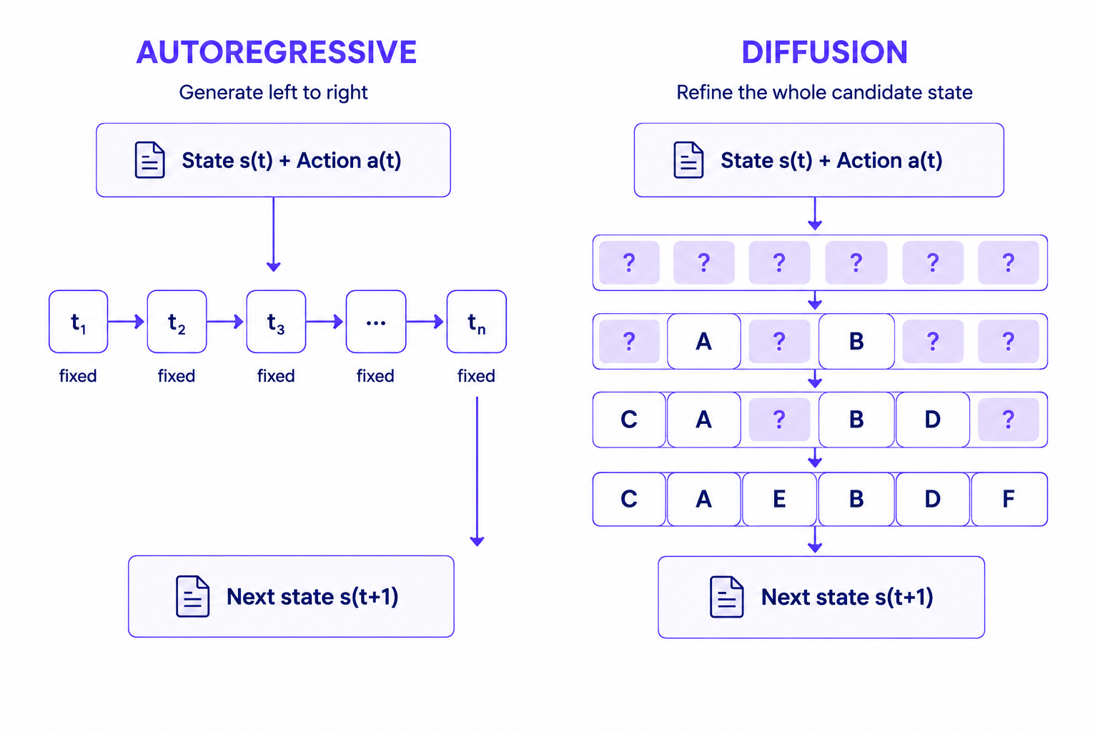
Autoregressive models generate one token at a time, with each token conditioned on the tokens that came before.
Consider an agent querying a database, and the world model needs to generate the resulting state. The schema for the tool call response in this example requires these specific fields: data_payload, processing_time, and status.
An autoregressive model generates this state strictly from left to right, one token at a time. It begins by predicting a successful-looking payload, perhaps hallucinating data based on the agent’s prompt, for example:
{
  "data_payload": {"user_id": 405, "name": "Sarah Connor"},
  "processing_time": "12ms",
As the model reaches the end of the sequence, it generates a correct but counter-logical status flag, resulting in this output:
{
  "data_payload": {"user_id": 405, "name": "Sarah Connor"},
  "processing_time": "12ms",
  "status": "error: unauthorized access"
}
This illustrates a possible failure mode of autoregressive generation. Because the response is generated from left to right, early fields are produced before later fields, such as “status,” are known. If the model commits to a successful-looking payload too early, it may later generate a status that is inconsistent with those earlier fields.
On the other hand, diffusion world models refine the whole tool call response jointly, allowing fields to influence one another during generation and reducing inconsistency risks, for example:
{
  "data_payload": null,
  "processing_time": "12ms",
  "status": "error: unauthorized access"
}
However, iterative denoising requires multiple model evaluations, so the inference cost depends on the number of denoising steps, the sequence length, and the implementation.
Anchoring as a key design feature
Autoregressive models can also be explicitly trained to fill gaps mid-sequence, as in the Fill-in-the-Middle approach, or to generate tokens regardless of order (XLNet), while constrained decoding forces the generation of valid JSON directly.
Fill-in-the-Middle techniques are typically rigid, designed to bridge a single gap rather than a scattered framework of constraints. Constrained decoding, while powerful, enforces only syntax; it cannot enforce semantic consistency. If an autoregressive model has already hallucinated a bad prefix, constrained decoding only forces it to wrap that bad logic in proper JSON. So what does diffusion actually add?
Diffusion treats any arbitrary combination of known fields as a native structural anchor; it doesn't rely on external parsers or rigid training hacks to enforce the rules. Because the model denoises the entire state simultaneously, it directs all predictive power toward making the unknown parts logically and semantically consistent with the anchors. It ensures that the generated values make sense within the fixed schema, rather than merely adhering to its format.
{{banner-large-dark-3="/banners"}}
Types of diffusion world models
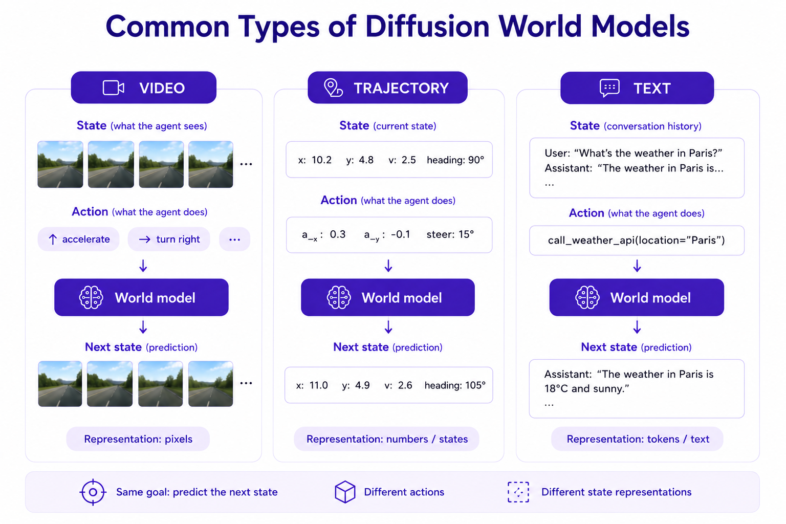
This article explores three types of diffusion world models: video, trajectory, and text.
Video world models
In this use case, world models predict the next frame of a scene, using an image as the state. The action in a video world model is a controlled input, such as a steering angle or a key press.
DIAMOND (Diffusion As a Model Of eNvironment Dreams) utilizes diffusion to train a reinforcement learning model inside a hallucinated simulation of an Atari video game. It uses high-fidelity image data as input, avoiding potential data loss during tokenization. It achieves a mean human-normalized score of 1.46 on the Atari 100k benchmark.
Another useful reference for video world models is Google DeepMind's Genie 2, a large-scale world model that generates action-controllable 3D worlds from a single image. Unlike DIAMOND, which is tied to one game's rule set, Genie 2 can spawn an entire world from a single input image. It also has long-horizon memory: it remembers parts of the world that leave the frame and renders them accurately when they return to view. Genie 2 is also used for rapid prototyping, since its out-of-distribution generalization lets you turn concept art and rough drawings into interactive environments.
Although previous reinforcement learning models could be applied to tasks similar to those they were trained on, large-scale generalization has remained a persistent issue for researchers.
DreamerV3 is a recurrent latent model (it keeps a compressed memory of the environment and updates it step by step), not a diffusion world model, but it's the reference point for scale here: the same algorithm and hyperparameters across 150+ tasks, from robot control to playing Minecraft and collecting diamonds from scratch, with no per-task tuning.
Dreamer 4 builds on DreamerV3 but replaces the recurrent network with a transformer-based dynamics model that uses flow matching and shortcut forcing, techniques closely related to diffusion-based generative modeling. Its world model can run in real time on a single GPU, and instead of calling a live environment, it learns its policy offline from recorded data. That is how it became the first agent to mine diamonds in Minecraft fully offline.
Trajectory world models
Rather than predicting pixels, trajectory world models predict states and rewards. Instead of relying on pixel-based representations, the environment is represented through compact numerical state variables, such as positions and velocities.
The Trajectory Diffusion World Model applies diffusion to motion sequences with a key advantage: it can predict multiple steps ahead in a single pass. The simultaneous calculation solves the prominent problem of compounding errors in traditional reinforcement learning.
In an autoregressive model, if an agent calculates the state at t+1, it must then feed that state back into itself to calculate the state at t+2, and so on; any inaccuracy in the first prediction compounds. By viewing the entire trajectory as a single canvas for the diffusion process, the model predicts the horizon jointly, mitigating the reliance on recursive one-step predictions.
On the D4RL (Datasets for Deep Data-Driven Reinforcement Learning) dataset, these models surpass one-step dynamics models by 44% and match or exceed their model-free counterparts.
Text world models
While the world models discussed previously in the article can simulate the physical world, text world models (TWMs) are commonly used to simulate digital environments.
Here, the environment is strictly text, such as a JSON response, a terminal buffer, a website's DOM, or conversation history. Given a conversation history and a tool-call definition, a text world model returns the expected response to the tool call.
Since text is discrete, these world models rely on masking rather than on the continuous Gaussian noise commonly used in image diffusion models. During training, these models take in an entire piece of text, a complete tool-call response, and mask specific tokens. This forces the model to infer what lies beneath the masked tokens using only the surrounding visible elements.
By repeating the process and varying the level of corruption, these models learn deep relationships between the environment and the input to the point that they can reconstruct an entire valid state from scratch.
Running inference is the exact opposite process. The model starts with a fully masked buffer and, instead of predicting the next word, it performs a rough pass over the entire sequence at once. Over several iterative passes, it sharpens the predictions, resulting in a fully coherent state. Since every denoising pass processes the entire sequence at once via bidirectional attention, all elements can interact with and correct one another, avoiding sequential-generation anomalies. In other words, the model is never forced to commit to a hallucinated prefix.
Alibaba demonstrated the scalability of this approach in 2026 by releasing Qwen-AgentWorld, which can simulate seven distinct digital environments within a single model via long chain-of-thought reasoning. Instead of acting purely as an agent, the model was trained to simulate the environment's responses across domains such as Terminals, Web, Software Engineering (SWE), MCP Tool Calling, Search, OS, and Android. However, training machine learning models on end-to-end systems involving these environments adds significant computational complexity and latency. Hence, this tool serves as a software-in-the-loop alternative that realistically mocks the actual tools.
It is important to note that while this article focuses on diffusion as the generative architecture, you can also implement text world models with other architectures, such as causal language models.
Training an agent against a diffusion world model
Once you have a world model, you can train an agent against it using the same general reinforcement learning loop as with the real environment: the agent acts, collects a reward, and updates its policy. The only change is that those responses come from the world model rather than the live tools and APIs.
Steering directives
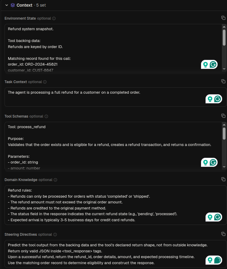
In agent training, a world model is particularly useful and distinct from a mock server because of its steering directives. World models are usually grounded by five distinct inputs before they can generate high-accuracy predictions.
- The Environment State: The system's current state.
- The Task Context: The conversation history or goal the agent is trying to achieve.
- The Tool Schemas: The API contracts the model must conform to.
- The Domain Rules: The physics of the underlying system (e.g., SQL constraints).
- The Steering Directives: Meta-instructions that dictate the simulation's dynamic behavior.
While the first four inputs define what is in the environment, the fifth defines how it behaves.
You can force the model to return a malformed JSON payload, hold back a crucial field the agent explicitly requested, or throw a sudden authentication error, simply to see how the agent handles the error. It can even replicate edge cases that are otherwise very difficult to reproduce in a production environment.
Rollout loop
During training, the agent and the environment interact in a continuous feedback loop, also known as a rollout loop.
- Agent acts
- Environment responds with the resulting state
- Agent acts again on the resulting state
The cycle repeats until the agent reaches the terminal state, at which point the finished trajectory is scored, and the agent's policy is updated. GRPO (Group Relative Policy Optimization) optimizes the agent’s policy by comparing the relative success of several attempts at the same task, scored against the group's average.
With digital world models, the agent interacts with the world model instead of the actual tool. The reward stays where it was; the world model predicts what the environment returns. It does not evaluate the agent itself.
See our guide to RL environments for GRPO and reward design.
Comparison with other training techniques
Researchers trained the same small agent four different ways, then counted how many ALFWorld tasks it could finish. ALFWorld is a text-based game: the agent reads a room description and types what to do next. The results, taken from this paper, are:
| Training technique | Tasks finished |
|---|---|
| Not trained | 5.7% |
| Supervised fine-tuning only | 42.9% |
| Fine-tuning, then reinforcement learning against an autoregressive world model | 48.6% |
| Fine-tuning, then reinforcement learning against a diffusion world model | 53.6% |
Both world models in the bottom two rows of the table above were trained on the same fine-tuning data. Although they used different base models and parameter counts, the diffusion approach clearly outperformed the autoregressive world model approach. In this specific ALFWorld setup, the diffusion-backed agent won by 5 percentage points, completing 5 more tasks per 100.
In the wider results, the performance gap can be much larger; for example, when testing a Mistral-7B-v0.3 agent on the ScienceWorld benchmark, the diffusion world model outperformed the autoregressive setup by over 15 percentage points.
Evaluating a diffusion world model
What to score
The very first and often most important thing to test for is realism.
- Does the response from the simulated system seem genuine?
- Does it adhere to the appropriate schema, formatting, and other system rules?
Secondly, did the system give the correct outcome? If the system looks correct but produces incorrect outcomes, it is still not realistically usable.
Thirdly, is the generated state actually worth learning from? Realistic states can still be uninformative or teach the wrong lessons.
The test that actually decides it
No matter how well your models score on these three questions or on your chosen metrics, the most valuable test of a simulation is generalization. If an agent trained on a simulated digital world model performs well on the actual system, then the model was well trained.
In other words, as in all machine learning, have a representative evaluation set ready for your model.
Simulating an agent environment with Patronus Digital World Model
Patronus AI builds infrastructure to develop, train, and evaluate AI agents. As agents develop from simple tasks to long-horizon projects, static evaluation datasets are no longer sufficient. To solve this, Patronus AI builds digital world models (DWM) where agents can practice, fail, and learn, all without risking real-world systems.
To see this in action, consider a scenario in which an AI customer support agent handles a return and executes a refund tool call. Normally, this request reaches out to a live payment provider and backend database. In this setup, Patronus DWM predicts the response on behalf of the real service. You can test this setup through DWM via a GUI-based playground or via a REST API.
DWM Playground
The DWM Playground is the quickest way to see what a digital world model does before you write any code.
Input panel
In the input panel, you can set parameters controlling the generative model itself:
- max_tokens - caps the number of response tokens to prevent overflow. A value like 4096 is often sufficient for typical tool-call scenarios.
- temperature - controls the randomness of the output (closer to 0 means more deterministic)
- top_p limits sampling to the smallest set of candidates whose cumulative probability reaches a chosen threshold.
- top_k limits sampling to the k most likely candidates.

Environment context
Then, define the environment context by providing the five inputs discussed earlier:
- The environmental state,
- The task context,
- The tool schemas,
- The domain rules,
- The steering directives.
All of these steps are shown in the following image.
Interaction
The next Interaction section requires two fields:
- State - The conversation so far, given as a list of chat messages.
- Action - The single step the agent is about to take: an assistant message carrying the tool call and its arguments.
Generate
Clicking Generate in the top-right corner of the screen generates a model response based on all the fields above, like this one.
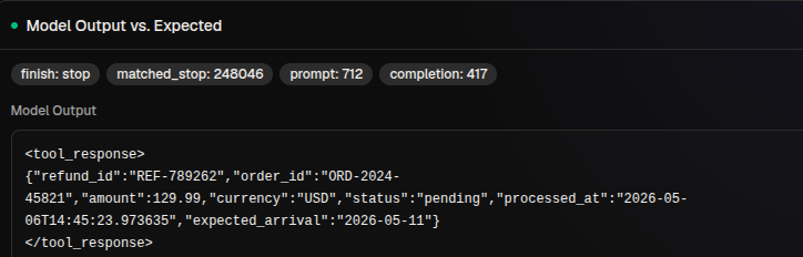
This is a valid tool-call response that conforms to the expected JSON schema and contains meaningful fields. To steer the response and simulate a timeout error in the service, it's enough to add a single steering command, such as: “The refund service should return a timeout error.”
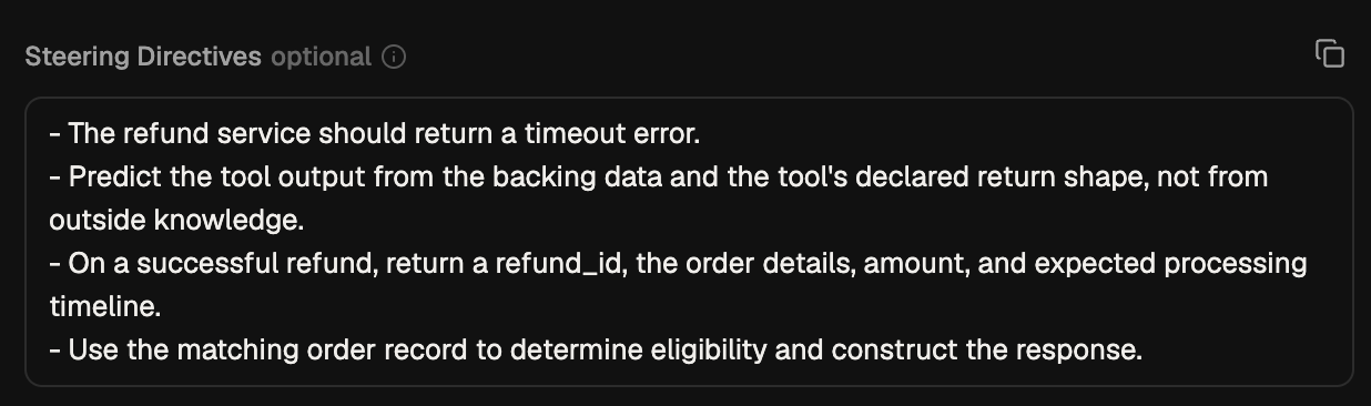
The model correctly picks up on this directive and generates the following result. Keep in mind that nothing else has been changed in the other parameters.
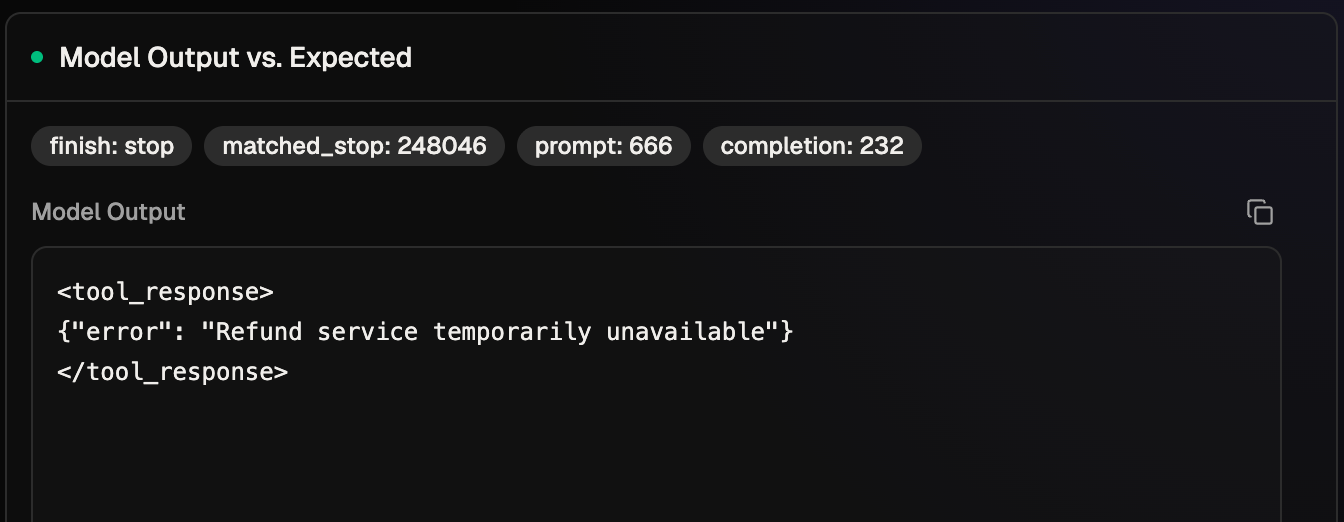
This was all done manually through the Patronus DWM Playground.
Using the REST API
World models can also be accessed programmatically via the Patronus DWM REST API. The API has two endpoints, both returning predictions from the same backend; they are just different API formats for developers' convenience.
The first native endpoint is `/predict`, while the second one is the OpenAI-compatible `/chat/completions`. To use either, you first need to get a Bearer API token from Patronus: https://dwm.patronus.ai/api-keys.
Here’s an example of calling the Patronus DWM API from Python. All of the code is available and runnable in this Google Colab Notebook.
Prerequisite: Authenticate
Before connecting to the API, set the authentication token you acquired from Patronus as a Google Colab secret. For the notebook to run without changes, name the secret `PATRONUS_DWM_API_KEY`.
import os, re, json, time
import requests
from google.colab import userdata

API_KEY = userdata.get('PATRONUS_DWM_API_KEY') # Make sure you have set PATRONUS_DWM_API_KEY in Google Colab
assert API_KEY, "Add PATRONUS_DWM_API_KEY in Colab's Secrets panel (key icon on the left sidebar) and grant this notebook access."

BASE_URL = "https://dwm.patronus.ai/v1"
HEADERS = {"Authorization": f"Bearer {API_KEY}", "Content-Type": "application/json"}
print("API key loaded from Colab secret PATRONUS_DWM_API_KEY.")
Step 1: Define the same variables as in the playground
In this example, the context variable is a dictionary that holds all five variables, with keys named the same as the fields in the playground.
order_id = "ORD-2024-45821"
original_amount = 129.99
currency = "USD"
This example defines reusable variables to automate validation in later steps.
context = {
   "environment_state": f"""
   - Tool backing data / query state:
 - Refunds are keyed by order ID.
- Matching record found for this call:
 - order_id: {order_id}
 - customer_id: CUST-8847
 - original_amount: {original_amount}
 - currency: {currency}
 - payment_method: credit_card
 - card_last_four: 4829
 - order_status: completed
 - order_date: 2024-01-15
 - refund_eligible: true
- Constraint shaping the result:
 - The refund amount matches the original transaction amount; no partial refund is requested.
   """,
   "task_context": "The agent is processing a full refund for a customer on a completed order.",
   "tool_schemas": """
- `process_refund`
 - Parameters:
   - `order_id`: string
   - `amount`: number
   - `reason`: string
 - Returns:
   - `{refund_id: string, order_id: string, amount: number, currency: string, status: string, processed_at: string, expected_arrival: string}`
 - Behavior:
   - Validates the order exists and is eligible for refund, then creates a refund transaction and returns a confirmation.
 - Error conditions:
   - Unknown order ID returns an error; ineligible orders (cancelled, already refunded) return an error.
   """,
   "domain_knowledge": """
   - Refunds can only be processed for orders with status 'completed' or 'shipped'.
- The refund amount must not exceed the original order amount.
- Refunds are credited to the original payment method.
- The status field in the response indicates the current refund state (e.g., 'pending', 'processed').
- Expected arrival is typically 3-5 business days for credit card refunds.
   """,
   "steering_directives": """
   - Predict the tool output from the backing data and the tool's declared return shape, not from outside knowledge.
- On a successful refund, return a refund_id, the order details, amount, and expected processing timeline.
- Use the matching order record to determine eligibility and construct the response.
"""
}

print("context sections set:", list(context.keys()))
The final line, the “context sections set” print, validates that all five variables are set correctly. Note that this example uses multiline strings for formatting, but single-line and multi-sentence strings work just as well.
Also, as in the playground, define the previous state and action messages as follows:
state_messages = [
   {"role": "user", "content": "I need to process a refund for order #ORD-2024-45821. The customer paid $129.99 and wants their money back."},
    {"role": "assistant", "content": "I'll process that refund for you right away."}
]

action_messages = [
   {"role": "assistant", "content": "", "tool_calls": [{"id": "call_78291463", "type": "function", "function": {"name": "process_refund", "arguments": "{\"order_id\": \"ORD-2024-45821\", \"amount\": 129.99, \"reason\": \"Customer request\"}"}}]}
]

interaction = {
   "state": json.dumps(state_messages),
   "action": json.dumps(action_messages),
}
This example intentionally places json.dumps() inside of the interaction. The API requires JSON-formatted strings, so Python dictionaries are serialized rather than manually written as JSON.
Step 2: Call the /predict endpoint
Forward all prepared data to the API and make the prediction. Define a `predict()` function that posts the request to the `/predict` endpoint.
def predict(context, interaction, params, timeout=180):
   """Call the native /predict endpoint and return the parsed JSON response."""
   resp = requests.post(
       f"{BASE_URL}/predict",
       headers=HEADERS,
       json={"context": context, "interaction": interaction, "params": params},
       timeout=timeout,
   )
   resp.raise_for_status()
   return resp.json()
Define the initial parameters set in the playground (max_tokens, temperature, top_p, top_k, and other parameters, such as whether thinking is enabled).
params = {
   "max_tokens": 4096, "temperature": 0.2, "top_p": 1, "top_k": 0,
   "enable_thinking": True, "reasoning_budget": "high",  # low=1024 | medium=4096 | high=8192 thinking tokens
}
Finally, call the predict endpoint with:
result = predict(context, interaction, params)Since thinking was enabled, the reasoning returns in a separate reasoning field on /predict; response.content above stays clean.
Step 3: Parse and verify the prediction
Define two separate functions: get_tool_response() to parse the JSON body from the <tool_response> tags, and verify() to assert that the refund, order ID, amount, and currency are returned correctly.
def get_tool_response(content: str) -> dict:
  """Extract the JSON object from the <tool_response> wrapper."""
  payload = re.search(r"<tool_response>\s*(\{.*\})\s*</tool_response>", content, re.DOTALL)
  if not payload:
    raise ValueError("No <tool_response> tag found in content")
  return json.loads(payload.group(1))

def verify(payload):
  """Verify if the tool response matches what we expected."""
  assert(payload.get("refund_id"))
  assert(payload.get("order_id") == order_id)
  assert(payload.get("amount") == original_amount)
  assert(payload.get("currency") == currency)
To invoke the two methods, nest the content inside the response object, further nested in the result object.
verify(get_tool_response(result.get("response").get("content")))If the response from the native endpoint contains all the attributes you are verifying, the function will not return a response. However, if an attribute is missing or doesn't match the expected value, the method throws an AssertionError.
Using the OpenAI API
Alternatively, if your data pipelines already use OpenAI-compatible endpoints, you can use the OpenAI library to format requests to the Patronus DWM base URL with your existing authentication token.
from openai import OpenAI

client = OpenAI(base_url=BASE_URL, api_key=API_KEY)

completion = client.chat.completions.create(
   model="world-model",
   messages=[],  # required by the SDK; ignored when world-model fields are present
   extra_body={
       "context": context,
       "interaction": interaction,
       "params": {"max_tokens": 4096, "temperature": 0.2,
                  "enable_thinking": True, "reasoning_budget": "high"},
   },
)

raw = completion.choices[0].message.content
The raw response is:
The agent calls process_refund with order_id "ORD-2024-45821", amount 129.99, and reason "Customer request".
The tool receives these parameters and first validates that the order exists in the backing data, finding the matching record for ORD-2024-45821.
The tool checks the order_status field, which is "completed", satisfying the domain rule that allows refunds for completed or shipped orders.
The tool also confirms refund_eligible is true and that the requested amount of 129.99 does not exceed the original_amount of 129.99, so no error is raised.
The tool creates a new refund transaction, assigning it the next available refund ID, which is REF-78291463, following the system's ID generation sequence.
The currency is taken directly from the order record as USD, and the amount is echoed back as 129.99.
The status is set to "pending" because the refund has been initiated but not yet fully processed through the payment network.
The processed_at timestamp is generated at the moment of the call, resolving to 2025-11-12T10:00:00Z.
The expected_arrival is computed as 3-5 business days from the processed_at date; the system selects the 3-day window, landing on 2025-11-17.
The tool serializes all these fields into a JSON response object and returns it to the agent.
</think>
<tool_response>
{"refund_id":"REF-78291463","order_id":"ORD-2024-45821","amount":129.99,"currency":"USD","status":"pending","processed_at":"2025-11-12T10:00:00Z","expected_arrival":"2025-11-17"}
</tool_response>
As you can see, the response ends with a </think> tag, followed by the actual tool response. The next code block removes the inline reasoning section and extracts only the relevant tool response.
The entire configuration (i.e. the same context, interaction, and params used in the native endpoint) is passed through the `extra_body` tag, formatted differently. The response is stored in the `raw` variable.
To verify output, parse `raw`:
def parse_thinking(text: str) -> str:
   """On /chat/completions, an enabled thinking pass is returned inline, ending with </think>."""
   return text.split("</think>")[-1].strip()

print("After parse_thinking(), then verified against the same rules")
tool_response = get_tool_response(parse_thinking(raw))
verify(tool_response)
Again, verify does not return a response if the API returns the expected output format. However, if the output lacks a required attribute or has an incorrect value for a required attribute, it raises an AssertionError. After calling get_tool_response(), the sanitized tool response is:
{'refund_id': 'REF-78291463', 'order_id': 'ORD-2024-45821', 'amount': 129.99, 'currency': 'USD', 'status': 'pending', 'processed_at': '2025-11-12T10:00:00Z', 'expected_arrival': '2025-11-17'}Modifying the steering directives
To steer the DWM, just set a new directive:
new_steering_directive = "The refund service refuses a response with a timeout error."
context["steering_directives"] = new_steering_directive


Or add one to the beginning:
new_steering_directive = "The refund service refuses a response with a timeout error."
context["steering_directives"] = new_steering_directive + context["steering_directives"]
{{banner-dark-small-3="/banners"}}
Final thoughts
Diffusion world models, as a field, are being applied across three main modalities: video world models for pixel processing, trajectory models for physical kinematics, and text models for digital systems.
The main advantage of this architecture is structural integrity. Empirical results show that diffusion-based world models outperformed the autoregressive world-model baseline by an average of 5.3 percentage points across configurations, with individual gaps reaching 15.1 percentage points, an advantage most pronounced in partially observable environments where complex latent states are not readily apparent to agents.
An autoregressive model must complete a sentence before seeing the rest of the sequence, often trapping itself in logical contradictions. Because diffusion world models refine the entire state simultaneously, the generated fields negotiate with one another, ensuring that the final predicted response is coherent.
For LLM-driven software agents, text diffusion models are the ideal sandbox.
You can try all of this yourself in the Patronus DWM Playground. Run your agent against a simulated environment instead of a live one, so a tool call never touches a real payment provider or database, and the failure cases you could never safely trigger in production, like timeouts or malformed responses, become easy to test.